This page was generated from docs/Examples/Sulf_Evolution_During_FC/Sulfide_sat_magma_evolution_Iceland.ipynb. Interactive online version: .

Python Notebook Download

Tracking sulfide saturation during magma evolution

• This Jupyter Notebook shows how to use the various functionalities of PySulfSat to track sulfide saturation during magma evolution

• This work is soon to be published as Liu et al. (in prep). You can download the data here: https://github.com/PennyWieser/PySulfSat/blob/main/docs/Examples/Sulf_Evolution_During_FC/Liu_Sulf_Compp.xlsx https://github.com/PennyWieser/PySulfSat/blob/main/docs/Examples/Sulf_Evolution_During_FC/HoluMIs.xlsx https://github.com/PennyWieser/PySulfSat/blob/main/docs/Examples/Sulf_Evolution_During_FC/Sulfide_compositions.xlsx https://github.com/PennyWieser/PySulfSat/blob/main/docs/Examples/Sulf_Evolution_During_FC/Model9_BaliOnlyLang_Closedsystem_32kbar_NiCu_02.xlsx

## First, if you havent alrready, install PySulfSat and Thermobar - remove # sign
#!pip install Thermobar
#!pip install PySulfSat

import matplotlib.pyplot as plt
import numpy as np
import pandas as pd
import PySulfSat as ss
import Thermobar as pt
pd.options.display.max_columns = None
print('Thermobar version')
print(pt.__version__)
print('PySulfSat version')
print(ss.__version__)

Thermobar version
1.0.17
PySulfSat version
0.0.17

Set some plotting parameters

plt.rcParams["font.size"] =12
plt.rcParams["mathtext.default"] = "regular"
plt.rcParams["mathtext.fontset"] = "dejavusans"
plt.rcParams['patch.linewidth'] = 1
plt.rcParams['axes.linewidth'] = 1
plt.rcParams["xtick.direction"] = "in"
plt.rcParams["ytick.direction"] = "in"
plt.rcParams["ytick.direction"] = "in"
plt.rcParams["xtick.major.size"] = 6 # Sets length of ticks
plt.rcParams["ytick.major.size"] = 4 # Sets length of ticks
plt.rcParams["ytick.labelsize"] = 12 # Sets size of numbers on tick marks
plt.rcParams["xtick.labelsize"] = 12 # Sets size of numbers on tick marks
plt.rcParams["axes.titlesize"] = 14 # Overall title
plt.rcParams["axes.labelsize"] = 14 # Axes labels

1. Load sulfide data

Sulfide_in=pd.read_excel('Liu_Sulf_Compp.xlsx')
Sulfide_in.head()

	Sample	Sulfide	Averaging method	S	Fe	Ni	Cu	Fe/(Fe+Cu+Ni)
0	H14	H14_S1	average (n=3)	34.365900	49.914425	2.323820	13.395820	0.760496
1	H14	H14_S2	average (n=3)	34.691202	50.071840	2.474618	12.762410	0.766693
2	H14	H14_S3	single	35.557799	56.234839	2.981762	5.225494	0.872641
3	H14	H14_S4	average (n=3)	33.705771	50.447033	2.400133	13.447063	0.760957
4	H14	H14_S5	average (n=3)	32.949899	45.135301	2.868397	19.046367	0.673158

H14_Sulf=Sulfide_in.loc[Sulfide_in['Sample']=="H14"]

2. Load best fit liquid line of descent

• This data is a Petrolog model

• The addition of the Liq suffix might seem a bit odd, but this allows use of liquid-only thermometers from the Python3 Thermobarometry tool Thermobar

Liqs=ss.import_data('Model9_BaliOnlyLang_Closedsystem_32kbar_NiCu_02.xlsx',
            Petrolog=True)
Liqs.head()

We have replaced all missing liquid oxides and strings with zeros.

	SiO2_Liq	TiO2_Liq	Al2O3_Liq	FeOt_Liq	MnO_Liq	MgO_Liq	CaO_Liq	Na2O_Liq	K2O_Liq	P2O5_Liq	H2O_Liq	Fe3Fet_Liq	Ni_Liq_ppm	Cu_Liq_ppm	SiO2_magma	TiO2_magma	Al2O3_magma	Fe2O3_magma	FeO_magma	MnO_magma	MgO_magma	CaO_magma	Na2O_magma	K2O_magma	P2O5_magma	Cr2O3_magma	H2O_magma	Ni_magma	Cu_magma	Cr2O3_Liq	Ni_Liq	Cu_Liq	SiO2_cumulate	TiO2_cumulate	Al2O3_cumulate	Fe2O3_cumulate	FeO_cumulate	MnO_cumulate	MgO_cumulate	CaO_cumulate	Na2O_cumulate	K2O_cumulate	P2O5_cumulate	Cr2O3_cumulate	H2O_cumulate	Ni_cumulate	Cu_cumulate	Temperature	Temperature_Olv	Temperature_Plg	Temperature_Cpx	Olv_Fo_magma	Olv_Kd	Plg_An_magma	Cpx_Mg#Cpx_magma	Olv_Fo_cumulate	Plg_An_cumulate	Cpx_Mg#Cpx_cumulate	Pressure(kbar)	Lg(fO2)	dNNO	density	Ln(viscosity)	Melt_%_magma	Olv_%_magma	Olv_Peritectic	Plg_%_magma	Plg_Peritectic	Cpx_%_magma	Cpx_Peritectic	Fluid_%_magma	Olv_%_cumulate	Plg_%_cumulate	Cpx_%_cumulate	Sample	Unnamed:73	Fe3+/FeT	T_K	P_kbar	Fraction_melt	Sample_ID_Liq
0	48.8740	0.7872	16.3903	7.638971	0.1413	10.1312	14.0169	1.5745	0.0606	0.0606	0.1514	0.099892	201.8	90.8	48.8740	0.7872	16.3903	0.8488	6.8759	0.1413	10.1312	14.0169	1.5745	0.0606	0.0606	0.0505	0.1514	201.8	90.8	0.0505	201.8	90.8	53.1146	0.2692	4.1113	0	3.4316	0	19.0162	19.8160	0.1718	0	0	0	0	524.7	19.1	1246.750	1239.978	1206.624	1246.750	-1.0	-1.0	-1.0	90.81	-1.0	-1.0	90.81	3.2	-8.45	-1.4	2.691	6.27	99.9900	0	N	0	N	0	N	0	0.0	0.0	0.0100	0.15	16:44:26	0.900028	1519.900	3.2	0.999900	0
1	48.8315	0.7924	16.5133	7.680913	0.1427	10.0416	13.9595	1.5885	0.0612	0.0612	0.1529	0.100341	198.6	91.6	48.8315	0.7924	16.5133	0.8573	6.9102	0.1427	10.0416	13.9595	1.5885	0.0612	0.0612	0.0510	0.1529	198.6	91.6	0.0510	198.6	91.6	53.1026	0.2707	4.1450	0	3.4620	0	19.0477	19.7294	0.1740	0	0	0	0	520.5	19.2	1243.719	1237.967	1209.133	1243.719	-1.0	-1.0	-1.0	90.69	-1.0	-1.0	90.75	3.2	-8.46	-1.4	2.691	6.32	98.9950	0	N	0	N	0	N	0	0.0	0.0	1.0050	0.15	16:44:26	0.899578	1516.869	3.2	0.989950	1
2	48.7880	0.7977	16.6394	7.723524	0.1442	9.9486	13.9021	1.6030	0.0618	0.0618	0.1545	0.100812	195.4	92.3	48.7880	0.7977	16.6394	0.8661	6.9449	0.1442	9.9486	13.9021	1.6030	0.0618	0.0618	0.0515	0.1545	195.4	92.3	0.0515	195.4	92.3	53.0900	0.2722	4.1797	0	3.4933	0	19.0788	19.6416	0.1762	0	0	0	0	516.3	19.2	1240.613	1235.861	1211.697	1240.613	-1.0	-1.0	-1.0	90.56	-1.0	-1.0	90.69	3.2	-8.48	-1.4	2.691	6.37	97.9904	0	N	0	N	0	N	0	0.0	0.0	2.0096	0.15	16:44:26	0.899107	1513.763	3.2	0.979904	2
3	48.7442	0.8031	16.7661	7.765925	0.1457	9.8541	13.8460	1.6175	0.0624	0.0624	0.1561	0.101292	192.2	93.0	48.7442	0.8031	16.7661	0.8750	6.9793	0.1457	9.8541	13.8460	1.6175	0.0624	0.0624	0.0520	0.1561	192.2	93.0	0.0520	192.2	93.0	53.0771	0.2736	4.2148	0	3.5249	0	19.1089	19.5545	0.1786	0	0	0	0	512.2	19.3	1237.493	1233.699	1214.267	1237.493	-1.0	-1.0	-1.0	90.43	-1.0	-1.0	90.62	3.2	-8.49	-1.3	2.692	6.41	96.9959	0	N	0	N	0	N	0	0.0	0.0	3.0041	0.15	16:44:26	0.898627	1510.643	3.2	0.969959	3
4	48.6995	0.8085	16.8958	7.808896	0.1472	9.7561	13.7900	1.6325	0.0631	0.0631	0.1577	0.101794	189.1	93.8	48.6995	0.8085	16.8958	0.8842	7.0140	0.1472	9.7561	13.7900	1.6325	0.0631	0.0631	0.0526	0.1577	189.1	93.8	0.0526	189.1	93.8	53.0635	0.2752	4.2509	0	3.5575	0	19.1387	19.4662	0.1810	0	0	0	0	508.0	19.4	1234.298	1231.436	1216.892	1234.298	-1.0	-1.0	-1.0	90.30	-1.0	-1.0	90.56	3.2	-8.51	-1.3	2.692	6.46	95.9923	0	N	0	N	0	N	0	0.0	0.0	4.0077	0.15	16:44:26	0.898125	1507.448	3.2	0.959923	4

## Because Ni and Cu are treated as trace elemnets, we can adjust their concentrations by a constant rather than having to rerun the models
Liqs['Ni_Liq_ppm']=Liqs['Ni_Liq_ppm']*1.1
Liqs['Cu_Liq_ppm']=Liqs['Cu_Liq_ppm']*(8/9)

Choosing a thermometer

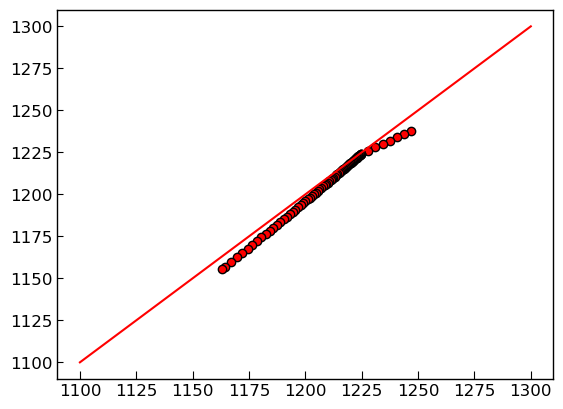
• Petrolog does have a temperature column, can also recalculate using Sugawara (A popular choice for Iceland), or Putirka (eq22 DMg). Putirka and Petrolog similar, lets just use Petrolog T for consistency.

Temp_Sugawara=pt.calculate_liq_only_temp(liq_comps=Liqs, equationT="T_Sug2000_eq3_ol", P=3.2)
Temp_Put=pt.calculate_liq_only_temp(liq_comps=Liqs, equationT="T_Put2008_eq22_BeattDMg", P=3.2)
plt.plot(Liqs['T_K']-273.15,Temp_Put-273.15, 'ok', mfc='r')
plt.plot([1100, 1300], [1100, 1300], '-r')

[<matplotlib.lines.Line2D at 0x2745fadf220>]

3. Loading in measured data to compare to models

• Here we load in matrix glasses and melt inclusion compositions, again, all data from Liu et al. (in prep).

# Melt inclusions from Bali et al.
BMI=pd.read_excel('HoluMIs.xlsx', sheet_name=' 3.Bali Supplement')
# Matrix glasses from Liu et al. (in prep)
LG=pd.read_excel('HoluMIs.xlsx', sheet_name='4.Liu Matrix Glass Data')

LG_14=LG.loc[LG['Comment'].str.contains('H4')]

8. SCSS models using predicted sulfide composition

• First, lets use the Smythe et al. (2017) model to predict sulfide compositions, based on petrolog Ni and Cu models

• As petrolog treates these incompatibly, we can multiply Ni and Cu by a constant, as if we had run the model with more Ni and Cu, withot having to do the calculations here. These fudge factors provide the best fit to observed Ni and Cu data.

Smythe_CalcSulf=ss.calculate_S2017_SCSS(df=Liqs, T_K=Liqs['T_K'],
P_kbar=3.2, Fe_FeNiCu_Sulf="Calc_Smythe",
Fe3Fet_Liq=Liqs['Fe3Fet_Liq'], Ni_Liq=Liqs['Ni_Liq_ppm'],
Cu_Liq=Liqs['Cu_Liq_ppm'])

• Now we use the Oneill (2021) model, first using their method for calculating sulfide composition, and then using the Smythe algorithm

ONeill_CalcSulf=ss.calculate_O2021_SCSS(df=Liqs, T_K=Liqs['T_K'],
P_kbar=3.2,
Fe_FeNiCu_Sulf="Calc_ONeill",
Ni_Liq=Liqs['Ni_Liq_ppm'],
Cu_Liq=Liqs['Cu_Liq_ppm'],
Fe3Fet_Liq=Liqs['Fe3Fet_Liq'])

ONeill_CalcSulf['Fe_FeNiCu_Sulf_calc'].head()

0    0.583722
1    0.586319
2    0.589038
3    0.591746
4    0.594277
Name: Fe_FeNiCu_Sulf_calc, dtype: float64

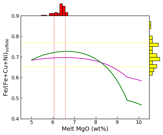
9. Lets compare these predictions to measured sulfide compositions

• For each sulfide, we have calculated an equivalent MgO content based on the melt or crystal it is hosted within

fig, (((ax3a),(ax3b)), ((ax4a, ax4b))) = plt.subplots(2, 2, figsize=(6,5),
                                    gridspec_kw={'height_ratios': [0.5, 4],
                                                 'width_ratios': [6, 0.5]
                                                })
plt.subplots_adjust(wspace=0, hspace=0)
ax3a.axis('off')
ax3b.axis('off')
ax4b.axis('off')

# Plot histogram of Mgo on ax3b
ax3a.hist(LG['MgO'],  ec='k', color='red')

# Plot histogram of sulifdes on ax3a
ax4b.hist(Sulfide_in['Fe/(Fe+Cu+Ni)'],  ec='k',
          color='yellow', orientation='horizontal', bins=15)
# Plot models on Ax4a
ax4a.plot([np.nanmean(LG['MgO'])-np.nanstd(LG['MgO']),
           np.nanmean(LG['MgO'])-np.nanstd(LG['MgO'])],
                                           [0.4, 0.9], '-r', lw=0.5)
ax4a.plot([np.nanmean(LG['MgO'])+np.nanstd(LG['MgO']),
           np.nanmean(LG['MgO'])+np.nanstd(LG['MgO'])],
                                           [0.4, 0.9], '-r', lw=0.5)

ax4a.plot([4.5, 11],
 [np.nanmean(Sulfide_in['Fe/(Fe+Cu+Ni)'])+np.nanstd(Sulfide_in['Fe/(Fe+Cu+Ni)']),
 np.nanmean(Sulfide_in['Fe/(Fe+Cu+Ni)'])+np.nanstd(Sulfide_in['Fe/(Fe+Cu+Ni)'])],
          '-', color='yellow', lw=0.5)

ax4a.plot([4.5, 11],
 [np.nanmean(Sulfide_in['Fe/(Fe+Cu+Ni)'])-np.nanstd(Sulfide_in['Fe/(Fe+Cu+Ni)']),
 np.nanmean(Sulfide_in['Fe/(Fe+Cu+Ni)'])-np.nanstd(Sulfide_in['Fe/(Fe+Cu+Ni)'])],
          '-', color='yellow', lw=0.5)

ax4a.plot(ONeill_CalcSulf['MgO_Liq'], ONeill_CalcSulf['Fe_FeNiCu_Sulf_calc'], '-m')
ax4a.plot(Smythe_CalcSulf['MgO_Liq'], Smythe_CalcSulf['Fe_FeNiCu_Sulf_calc'], '-g')


ax3a.set_xlim([4.5, 10.5])
ax4a.set_xlim([4.5, 10.5])
ax4b.set_ylim([0.4, 0.9])
ax4a.set_ylim([0.4, 0.9])
ax4a.set_xlabel('Melt MgO (wt%)')
ax4a.set_ylabel('Fe/(Fe+Cu+Ni)$_{sulfide}$')
fig.savefig('SulfComp.png', dpi=200)
# Plot a fill between

Performing calculations using average measured sulfide content

Smythe_MeasSulf=ss.calculate_S2017_SCSS(df=Liqs, T_K=Liqs['T_K'],
    Fe3Fet_Liq=Liqs['Fe3Fet_Liq'],
P_kbar=3.2, Fe_FeNiCu_Sulf=np.nanmean(Sulfide_in['Fe/(Fe+Cu+Ni)']))

Using inputted Fe_FeNiCu_Sulf ratio for calculations.
no non ideal SCSS as no Cu/CuFeNiCu

ONeill_MeasSulf=ss.calculate_O2021_SCSS(df=Liqs, T_K=Liqs['T_K'],
P_kbar=3.2,
Fe_FeNiCu_Sulf=np.nanmean(Sulfide_in['Fe/(Fe+Cu+Ni)']),
Fe3Fet_Liq=Liqs['Fe3Fet_Liq'])

Using inputted Fe_FeNiCu_Sulf ratio for calculations.

# bit of S6+
s6_corr_10=1/(1-10/100)
s6_corr_10

1.1111111111111112

Calculating fractional crystallization path

S_init=790
Calc_S_incom=ss.crystallize_S_incomp(S_init=S_init, F_melt=Liqs['Melt_%_magma']/100)
Calc_S_incom.head()

0    790.079008
1    798.020102
2    806.201424
3    814.467416
4    822.982677
Name: Melt_%_magma, dtype: float64

Calculating amount of sulfide removed

S_Sulf=np.nanmean(H14_Sulf['S'])*10000
S_Sulf_Err=np.std(H14_Sulf['S'])*10000


S_Rem_ON_S2=ss.calculate_mass_frac_sulf(S_model=ONeill_MeasSulf['SCSS2_ppm'],
                               S_init=S_init,
                               F_melt=Liqs['Melt_%_magma']/100,
                               S_sulf=S_Sulf)
S_Rem_ON_S6=ss.calculate_mass_frac_sulf(S_model=ONeill_MeasSulf['SCSS2_ppm']*s6_corr_10,
                               S_init=S_init,
                               F_melt=Liqs['Melt_%_magma']/100,
                               S_sulf=S_Sulf)
S_Rem_Smythe=ss.calculate_mass_frac_sulf(S_model=Smythe_MeasSulf['SCSS2_ppm_ideal_Smythe2017'],
                               S_init=S_init,
                               F_melt=Liqs['Melt_%_magma']/100,
                               S_sulf=S_Sulf)

# Minus 1 sigma, if also do sigma on S, min value, max S in sulf
S_Rem_Smythe_minus1sig=ss.calculate_mass_frac_sulf(
S_model=Smythe_MeasSulf['SCSS2_ppm_ideal_Smythe2017']-
Smythe_MeasSulf['SCSS2_ppm_ideal_Smythe2017_1sigma'],
S_init=S_init,
F_melt=Liqs['Melt_%_magma']/100,
S_sulf=S_Sulf-S_Sulf_Err)


S_Rem_Smythe_plus1sig=ss.calculate_mass_frac_sulf(
S_model=Smythe_MeasSulf['SCSS2_ppm_ideal_Smythe2017']+
Smythe_MeasSulf['SCSS2_ppm_ideal_Smythe2017_1sigma'],
                               S_init=S_init,
                               F_melt=Liqs['Melt_%_magma']/100,
S_sulf=S_Sulf+S_Sulf_Err)

# To convert from mass to volume
M_Factor=(2804/4200)

## Rset of the plots
fig, ((ax0, ax1), (ax2, ax3)) = plt.subplots(2,2, figsize = (12,10)) # adjust dimensions of figure here

# Fixed sulfide
ax0.plot(LG['MgO'], LG['S'], '^k', mfc='red', ms=6)
ax0.plot(BMI['MgO'], BMI['S-ppm'], 'ok', mfc='blue', ms=6)
ax0.plot(Liqs['MgO_Liq'], Calc_S_incom, '-k')
ax0.plot(ONeill_MeasSulf['MgO_Liq'], ONeill_MeasSulf['SCSS2_ppm'],
         '-m')
ax0.plot(Smythe_MeasSulf['MgO_Liq'], Smythe_MeasSulf['SCSS2_ppm_ideal_Smythe2017'],
         '-g')
ax0.plot(Smythe_MeasSulf['MgO_Liq'], s6_corr_10*Smythe_MeasSulf['SCSS2_ppm_ideal_Smythe2017'],
         ':g')
xfill=Smythe_MeasSulf['MgO_Liq']
y2fill_pap=(Smythe_MeasSulf['SCSS2_ppm_ideal_Smythe2017']+
Smythe_MeasSulf['SCSS2_ppm_ideal_Smythe2017_1sigma'])
y1fill_pap=(Smythe_MeasSulf['SCSS2_ppm_ideal_Smythe2017']-
Smythe_MeasSulf['SCSS2_ppm_ideal_Smythe2017_1sigma'])
ax0.fill_between(xfill, y1fill_pap, y2fill_pap,
                 where=y1fill_pap < y2fill_pap, interpolate=True,
                 color='green', alpha=0.1)

# Calculated sulfide
ax1.plot(LG['MgO'], LG['S'], '^k', mfc='red', ms=6)
ax1.plot(BMI['MgO'], BMI['S-ppm'], 'ok', mfc='blue', ms=6)
ax1.plot(Liqs['MgO_Liq'], Calc_S_incom, '-k')
ax1.plot(ONeill_CalcSulf['MgO_Liq'], ONeill_CalcSulf['SCSS2_ppm'],
         '-m')
ax1.plot(Smythe_CalcSulf['MgO_Liq'], Smythe_CalcSulf['SCSS2_ppm_ideal_Smythe2017'],
         '-g')
ax1.plot(Smythe_CalcSulf['MgO_Liq'], s6_corr_10*Smythe_CalcSulf['SCSS2_ppm_ideal_Smythe2017'],
         ':g')
xfill=Smythe_CalcSulf['MgO_Liq']
y2fill_pap=(Smythe_CalcSulf['SCSS2_ppm_ideal_Smythe2017']+
Smythe_CalcSulf['SCSS2_ppm_ideal_Smythe2017_1sigma'])
y1fill_pap=(Smythe_CalcSulf['SCSS2_ppm_ideal_Smythe2017']-
Smythe_CalcSulf['SCSS2_ppm_ideal_Smythe2017_1sigma'])
ax1.fill_between(xfill, y1fill_pap, y2fill_pap,
                 where=y1fill_pap < y2fill_pap, interpolate=True, ec=None,
                 color='green', alpha=0.1)

## Amount of sulfide fractionated
ax2.plot(Liqs['MgO_Liq'], 100*S_Rem_ON_S2*M_Factor, '-g')
ax2.plot(Liqs['MgO_Liq'], 100*S_Rem_ON_S6*M_Factor, ':g')
ax2.plot(Liqs['MgO_Liq'], 100*S_Rem_Smythe*M_Factor, '-m')
xfill=Liqs['MgO_Liq']
y2fill_pap=100*S_Rem_Smythe_minus1sig*M_Factor
y1fill_pap=100*S_Rem_Smythe_plus1sig*M_Factor
ax2.fill_between(xfill, y1fill_pap, y2fill_pap,
                 where=y1fill_pap < y2fill_pap, interpolate=True, ec=None,
                 color='green', alpha=0.1)
ax2.set_ylim([0, 0.1])
ax2.errorbar(np.nanmean(LG_14['MgO']),
             0.07,
             xerr=np.nanstd(LG_14['MgO']),
             yerr=0.03,
           fmt='d', ecolor='k', elinewidth=0.8, mfc='cyan', ms=10, mec='k', capsize=5)

ax0.set_xlabel('Melt MgO (wt%)')
ax0.set_ylabel('Melt S (ppm)')
ax1.set_xlabel('Melt MgO (wt%)')
ax1.set_ylabel('Melt S (ppm)')
ax2.set_xlabel('Melt MgO (wt%)')
ax2.set_ylabel('Vol % Sulfide')
ax2.set_ylim([0, 0.15])
plt.subplots_adjust( hspace=0.3)
fig.savefig('Sulf_frac.png', dpi=200)