This page was generated from docs/Examples/Mantle_Melting_Lee_Wieser/Complex_melt_changing_SCSS.ipynb. Interactive online version: .

Calculating sulfur and trace element evolution during mantle melting with changing SCSS and KDs

This notebook shows how to use the mantle melting model of Lee et al. (2012) adapted by Wieser et al. (2020) to model how S, Cu and other chalcophile or lithophile elements evolve during mantle melting
For more information on how the math works, we direct you towards the supporting information of Wieser et al (2020) - https://doi.org/10.1016/j.gca.2020.05.018 - Where the equations are typed out in detail
Here, we do the more complex example where silicate modes change and SCSS and KD change

Loading libraries

[1]:

import numpy as np
import pandas as pd
import matplotlib.pyplot as plt
import PySulfSat as ss

Example 1 - Non fixed S content

The examples in the other workbook assume that S is fixed throughout the melting interval
However, we know the concentration of mantle melts changes with increasing F, so ideally, we’d calculate how much S those melts can hold
We can do this using an output from a melting model (here, Thermocalc).

[2]:

# Load a generic dataframe
Thermocalc_df=pd.read_excel('Thermocalc_Melting_Path.xlsx')

[3]:

# Load a dataframe for calculating SCSS for these melt comps
Thermo_df_ss=ss.import_data('Thermocalc_Melting_Path.xlsx',
                    suffix='_Liq')

We have replaced all missing liquid oxides and strings with zeros.

Calculate instanteous melts

This dataframe contains aggregated melt compositions, we need instantenous melts for calculating the SCSS

[4]:

Inst_Liq=ss.calculate_inst_melts_Thermocalc(Thermocalc_df=Thermocalc_df)
Inst_Liq.head()

[4]:

	SiO2_Liq	Al2O3_Liq	CaO_Liq	MgO_Liq	FeO_Liq	Na2O_Liq	Fe2O3_Liq	FeOt_Liq
0	48.30	15.09	10.22	12.50	9.40	3.88	0.54	9.885892
1	48.20	15.07	10.35	12.57	9.41	3.80	0.52	9.877896
2	48.02	15.01	10.59	12.71	9.43	3.62	0.50	9.879900
3	47.84	14.98	10.86	12.88	9.45	3.47	0.48	9.881904
4	47.66	14.90	11.08	13.00	9.47	3.31	0.46	9.883908

TiO\(_2\) is very bad from Thermocalc, lets calculate it using our melting functions here

[5]:

KDs_TiO2=pd.DataFrame(data={'element': 'TiO2',
        'ol': 0.07, 'opx': 0.07,
        'cpx': 0.07, 'sp': 0.07,
        'gt': 0.07, 'sulf': 0.07}, index=[0])

Extract the modes from Thermocalc

[6]:

Modes3=pd.DataFrame(data={'ol': Thermocalc_df['ol'],
                        'cpx': Thermocalc_df['cpx'],
                        'opx': Thermocalc_df['opx'],
                        'sp': Thermocalc_df['sp'],
                        'gt': Thermocalc_df['g']*0})

[7]:

df_TiO2_Thermocalc=ss.Lee_Wieser_sulfide_melting(F=Thermocalc_df['liq'],
                        Modes=Modes3,
                        KDs=KDs_TiO2,
                        S_Sulf=330000, elem_Per=0.13,
                        S_Mantle=[200],
                        S_Melt_SCSS_2_ppm=1000,
                         Prop_S6=0)
Inst_Liq['TiO2_Liq']=df_TiO2_Thermocalc['TiO2_Melt_Inst']

Lets calculate the SCSS using ONeill (2021)

Wieser et al. (2020) show that the calculated sulfide composition isn’t very reliable at mantle PT, so we use a fixed mantle S composition of Fe/(Fe+Ni+Cu)=0.634

[8]:

SCSS_fixedSulf=ss.calculate_O2021_SCSS(df=Inst_Liq,
T_K=Thermocalc_df['T']+273.15, P_kbar=Thermocalc_df['P'],
Fe_FeNiCu_Sulf=0.634)
SCSS_fixedSulf.head()

Using inputted Fe_FeNiCu_Sulf ratio for calculations.

[8]:

	SCSS2_ppm	LnS	Ln_a_FeO	Ln_a_FeS	DeltaG	LnCS2_calc	SiO2_Liq	Al2O3_Liq	CaO_Liq	MgO_Liq	FeO_Liq	Na2O_Liq	Fe2O3_Liq	FeOt_Liq	TiO2_Liq	Fe_FeNiCu_Sulf_calc
0	1044.741097	6.951524	-2.187206	-0.532776	6.105676	-0.808582	48.30	15.09	10.22	12.50	9.40	3.88	0.54	9.885892	0.000000	0.634
1	1103.032862	7.005819	-2.246978	-0.531748	6.098787	-0.808198	48.20	15.07	10.35	12.57	9.41	3.80	0.52	9.877896	1.860432	0.634
2	1116.546495	7.017996	-2.245749	-0.531987	6.091909	-0.787675	48.02	15.01	10.59	12.71	9.43	3.62	0.50	9.879900	1.613651	0.634
3	1131.497103	7.031297	-2.244104	-0.532091	6.085093	-0.765808	47.84	14.98	10.86	12.88	9.45	3.47	0.48	9.881904	1.396916	0.634
4	1146.297359	7.044292	-2.243501	-0.532328	6.078288	-0.745169	47.66	14.90	11.08	13.00	9.47	3.31	0.46	9.883908	1.206812	0.634

Now we are ready to model S-Cu

instead of inputting a single value for S_melt_SCSS_2_ppm, we input the pandas dataframe.

[9]:

KDs_Cu=pd.DataFrame(data={'element': 'Cu',
        'ol': 0.048, 'opx': 0.034,
        'cpx': 0.043, 'sp': 0.223,
        'gt': 0, 'sulf': 800}, index=[0])

Modes=pd.DataFrame(data={'ol': 0.6, 'opx': 0.2,
       'cpx': 0.18, 'sp': 0.02, 'gt': 0}, index=[0])

# Lets run the simple model for comparison
S_Sulf = 38*(10**4)
df_Cu_200S=ss.Lee_Wieser_sulfide_melting(F=Thermocalc_df['liq'],
                        Modes=Modes,
                        KDs=KDs_Cu,
                        S_Sulf=S_Sulf, elem_Per=30,
                        S_Mantle=[200],
                        S_Melt_SCSS_2_ppm=1000,
                         Prop_S6=0)
# Now lets change S

df_Cu_200S_Thermocalc=ss.Lee_Wieser_sulfide_melting(F=Thermocalc_df['liq'],
                        Modes=Modes3,
                        KDs=KDs_Cu,
                        S_Sulf=S_Sulf, elem_Per=30,
                        S_Mantle=[200],
                        S_Melt_SCSS_2_ppm=SCSS_fixedSulf['SCSS2_ppm'],
                         Prop_S6=0)

[10]:

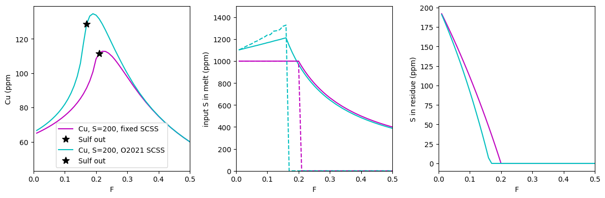
fig, ((ax1, ax2, ax3)) = plt.subplots(1, 3, figsize=(12,4), sharex=True)
# 100 ppm
ax1.plot(df_Cu_200S['F'].iloc[1:],
         df_Cu_200S['Cu_Melt_Agg'].iloc[1:],
        '-',color='m', ms=10, label='Cu, S=200, fixed SCSS')
# Lets add a cross to show the point at which sulfide is exhausted
sulf_out_200=np.take(np.where(df_Cu_200S['S_Residue']==0), 0)
ax1.plot(df_Cu_200S['F'].loc[sulf_out_200],
         df_Cu_200S['Cu_Melt_Agg'].loc[sulf_out_200],
        '*k', ms=10, label='Sulf out')


ax1.plot(df_Cu_200S_Thermocalc['F'].iloc[1:],
         df_Cu_200S_Thermocalc['Cu_Melt_Agg'].iloc[1:],
        '-',color='c', ms=10, label='Cu, S=200, O2021 SCSS')
# Lets add a cross to show the point at which sulfide is exhausted
sulf_out_200=np.take(np.where(df_Cu_200S_Thermocalc['S_Residue']==0), 0)
ax1.plot(df_Cu_200S_Thermocalc['F'].loc[sulf_out_200],
         df_Cu_200S_Thermocalc['Cu_Melt_Agg'].loc[sulf_out_200],
        '*k', ms=10, label='Sulf out')
ax1.set_xlim([0, 0.5])
ax1.set_xlabel('F')
ax1.set_ylabel('Cu (ppm')

# Plot S in melt
ax2.plot(df_Cu_200S['F'].iloc[1:],
         df_Cu_200S['S_Melt_Agg'].iloc[1:],
        '-',color='m', ms=10, label='Cu, S=200, fixed SCSS')

ax2.plot(df_Cu_200S_Thermocalc['F'].iloc[1:],
         df_Cu_200S_Thermocalc['S_Melt_Agg'].iloc[1:],
        '-',color='c', ms=10, label='Cu, S=200, O2021 SCSS')





ax2.set_xlabel('F')
ax2.set_ylabel('input S in melt (ppm)')

# S in source
ax3.plot(df_Cu_200S['F'].iloc[1:],
         df_Cu_200S['S_Residue'].iloc[1:],
        '-',color='m', ms=10, label='Cu, S=200, fixed SCSS')

ax3.plot(df_Cu_200S_Thermocalc['F'].iloc[1:],
         df_Cu_200S_Thermocalc['S_Residue'].iloc[1:],
        '-',color='c', ms=10, label='Cu, S=200, O2021 SCSS')

ax3.set_xlabel('F')
ax3.set_ylabel('S in residue (ppm)')
fig.tight_layout()
ax1.legend()
ax2.set_ylim([0, 1500])

[10]:

(0.0, 1500.0)

../../_images/Examples_Mantle_Melting_Lee_Wieser_Complex_melt_changing_SCSS_17_1.png

Example 2 - Variable KD

We can be even ‘cleverer’ than this. So far, we have assumed the KDs stay constant, but that isn’t the case. We know from Kiseeva et al. (2015) that the KD of Cu in the sulfide depends on the FeOt content of the melt, the sulfide composition and the temperature.
Following Ding and Dasgupta, lets calculate KD using 5 wt% Cu and 20 wt% Ni in the mantle sulfide

Calculate KD using Kiseeva, using a fixed sulfide composition.

[11]:

Sulf_KDs_Kis=ss.calculate_sulf_kds(Ni_Sulf=5, Cu_Sulf=20,
        FeOt_Liq=Thermocalc_df['FeOt'],
        T_K=Thermocalc_df['T']+273.15, Fe3Fet_Liq=0)
Sulf_KDs_Kis.head()

[11]:

	S_Sulf	O_Sulf	Fe_Sulf	Ni_Sulf	Cu_Sulf	DNi	DCu	DAg	DPb	DZn	...	DIn	DTi	DGa	DSb	DCo	DV	DGe	DCr	DSe_B2015	DTe_B2015
0	28.951975	2.040467	44.007558	5	20	468.888700	423.437545	387.173238	24.179410	2.000184	...	13.909661	0.009705	0.069138	31.618608	33.696187	0.213793	1.418172	1.365763	1194.743950	11164.888225
1	28.954668	2.038823	44.006509	5	20	467.544755	421.716344	385.632376	24.167264	2.003319	...	13.914218	0.009722	0.069545	31.714442	33.678820	0.214521	1.425514	1.369429	1195.816660	11175.374871
2	28.954331	2.039029	44.006641	5	20	465.786726	419.721374	383.854833	24.132319	2.004770	...	13.901989	0.009734	0.069894	31.771584	33.629184	0.215073	1.430966	1.371968	1195.682200	11174.060687
3	28.953993	2.039235	44.006772	5	20	464.050446	417.753198	382.100957	24.097713	2.006208	...	13.889863	0.009746	0.070241	31.828280	33.580030	0.215621	1.436388	1.374488	1195.547751	11172.746524
4	28.953656	2.039441	44.006904	5	20	462.323330	415.797345	380.357852	24.063208	2.007645	...	13.877764	0.009758	0.070590	31.884979	33.531021	0.216170	1.441821	1.377008	1195.413312	11171.432383

5 rows × 23 columns

Now lets make a dataframe of KDs

You could also set the silicate KDs to vary based on any other Kd models you have for them in the same way as above/

[12]:

KDs_Cu_Kis=pd.DataFrame(data={'element': 'Cu',
        'ol': 0.048, 'opx': 0.034,
        'cpx': 0.043, 'sp': 0.223,
        'gt': 0, 'sulf': Sulf_KDs_Kis['DCu']})

[13]:

fig, ((ax1, ax2, ax3)) = plt.subplots(1, 3, figsize=(10,4))

ax1.plot(Thermocalc_df['liq'],
         Sulf_KDs_Kis['DCu'], '-k')
ax1.set_xlabel('F')
ax1.set_ylabel('D$_{Cu}$')

ax2.plot(Thermocalc_df['FeOt'],
         Sulf_KDs_Kis['DCu'], '-k')
ax2.set_xlabel('FeOt')
ax2.set_ylabel('D$_{Cu}$')

ax3.plot(Thermocalc_df['T'],
         Sulf_KDs_Kis['DCu'], '-k')
ax3.set_xlabel('T')
ax3.set_ylabel('D$_{Cu}$')
fig.tight_layout()

../../_images/Examples_Mantle_Melting_Lee_Wieser_Complex_melt_changing_SCSS_23_0.png

[14]:

df_Cu_200S_Thermocalc_Kis=ss.Lee_Wieser_sulfide_melting(F=Thermocalc_df['liq'],
                        Modes=Modes3,
                        KDs=KDs_Cu_Kis,
                        S_Sulf=S_Sulf, elem_Per=30,
                        S_Mantle=[200],
                        S_Melt_SCSS_2_ppm=SCSS_fixedSulf['SCSS2_ppm'],
                         Prop_S6=0)

# Lets also model Selenium
df_Cu_200S_Thermocalc_Kis=ss.Lee_Wieser_sulfide_melting(F=Thermocalc_df['liq'],
                        Modes=Modes3,
                        KDs=KDs_Cu_Kis,
                        S_Sulf=S_Sulf, elem_Per=30,
                        S_Mantle=[200],
                        S_Melt_SCSS_2_ppm=SCSS_fixedSulf['SCSS2_ppm'],
                         Prop_S6=0)

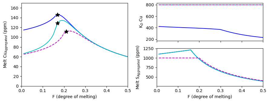
[15]:

#fig, ((ax1, ax2), (ax3, ax4)) = plt.subplots(2, 2, figsize=(10,8))
figure_mosaic="""
    AB
    AC

    """
fig,axes=plt.subplot_mosaic(mosaic=figure_mosaic, figsize=(9, 3.5), sharex=True)

axes['A'].plot(df_Cu_200S['F'].iloc[1:],
         df_Cu_200S['Cu_Melt_Agg'].iloc[1:],
        '--',color='m', ms=10, label='Cu, S=200 ppm, simple')
# Lets add a cross to show the point at which sulfide is exhausted
sulf_out_200=np.take(np.where(df_Cu_200S['S_Residue']==0), 0)
axes['A'].plot(df_Cu_200S['F'].loc[sulf_out_200],
         df_Cu_200S['Cu_Melt_Agg'].loc[sulf_out_200],
        '*k', ms=10, label='Sulf out')




# Kiseeva KDs, O2021 SCSS
axes['A'].plot(df_Cu_200S_Thermocalc_Kis['F'].iloc[1:],
         df_Cu_200S_Thermocalc_Kis['Cu_Melt_Agg'].iloc[1:],
        '-',color='b', ms=10, label='Cu, S=200 ppm, Kiseeva KDs, O2021 SCSS')
# Lets add a cross to show the point at which sulfide is exhausted
sulf_out_200=np.take(np.where(df_Cu_200S_Thermocalc_Kis['S_Residue']==0), 0)
axes['A'].plot(df_Cu_200S_Thermocalc_Kis['F'].loc[sulf_out_200],
         df_Cu_200S_Thermocalc_Kis['Cu_Melt_Agg'].loc[sulf_out_200],
        '*k', ms=10, label='Sulf out')

# FixedKD, O2021 SCSS

axes['A'].plot(df_Cu_200S_Thermocalc['F'].iloc[1:],
         df_Cu_200S_Thermocalc['Cu_Melt_Agg'].iloc[1:],
        '-',color='c', ms=10, label='Cu, S=200, KD=800, O2021 SCSS')
# Lets add a cross to show the point at which sulfide is exhausted
sulf_out_200=np.take(np.where(df_Cu_200S_Thermocalc['S_Residue']==0), 0)
axes['A'].plot(df_Cu_200S_Thermocalc['F'].loc[sulf_out_200],
         df_Cu_200S_Thermocalc['Cu_Melt_Agg'].loc[sulf_out_200],
        '*k', ms=10, label='Sulf out')
axes['A'].set_xlim([0, 0.5])
axes['A'].set_xlabel('F (degree of melting)')
axes['A'].set_ylabel('Melt Cu$_{Aggregated}$ (ppm)')
axes['A'].set_ylim([0, 170])


axes['B'].plot(df_Cu_200S_Thermocalc_Kis['F'].iloc[1:],
               KDs_Cu_Kis['sulf'].iloc[1:], '-b')
axes['B'].plot(df_Cu_200S_Thermocalc['F'].iloc[1:],
               df_Cu_200S_Thermocalc['F'].iloc[1:]*0+800, '-c')
axes['B'].plot(df_Cu_200S['F'].iloc[1:],
               df_Cu_200S['F'].iloc[1:]*0+800, '--m')
axes['B'].set_ylabel('K$_D$ Cu')

axes['C'].plot(df_Cu_200S_Thermocalc_Kis['F'].iloc[1:],
               df_Cu_200S_Thermocalc_Kis['S_Melt_Agg'].iloc[1:], '-b')
axes['C'].plot(df_Cu_200S_Thermocalc['F'].iloc[1:],
               df_Cu_200S_Thermocalc['S_Melt_Agg'].iloc[1:], '-c')
axes['C'].plot(df_Cu_200S['F'].iloc[1:],
               df_Cu_200S['S_Melt_Agg'].iloc[1:], '--m')



axes['C'].set_xlabel('F (degree of melting)')
axes['C'].set_ylabel('Melt S$_{Aggregated}$ (ppm)')
fig.tight_layout()
fig.savefig('Complex_Models.png', dpi=300)

../../_images/Examples_Mantle_Melting_Lee_Wieser_Complex_melt_changing_SCSS_25_0.png

[16]:

plt.plot(df_Cu_200S_Thermocalc['F'].iloc[1:],
               df_Cu_200S_Thermocalc['S_Melt_Agg'].iloc[1:], '-c')

[16]:

[<matplotlib.lines.Line2D at 0x17dd803baf0>]

../../_images/Examples_Mantle_Melting_Lee_Wieser_Complex_melt_changing_SCSS_26_1.png

[ ]:

[ ]: